

Let the Traveling Salesman Optimize your Power Station
In this optimization article, I explain how to simplify a nonlinear power plant dispatch problem into a standard Traveling Salesman Problem that anyone can work. Level: Intermediate. Time: 15 min.
Starting up
A thermal power station — a gas or a coal burner — is more than a giant cash machine. It is a giant machine, a real option. You run it when profitable and switch it off when unprofitable. And as you would imagine, several hundred million euros worth of power plant is more complicated than a light switch. Oil burners must preheat the main boilers to a sufficient temperature. Coal must be pulverized. In some cases, gas capacity must be scheduled. This takes time and a lot of money. Starting up a station is a big commitment.
To help utilities make the most profitable startup and shut-down decisions, we rely on optimization algorithms to give us a pretty good schedule for how to run our assets with a given price forecast.
The Slow Approach
If we merely wanted to optimize our station’s run-schedule with the current prices as fixed inputs, we could allow ourselves the luxury of solving a slow, bulky non-linear optimization problem. This model could include all the bells and whistles: nonlinear fuel efficiency curves as a function of output and temperature; differentiation between cold starts and warm starts; nonlinear jumps of output between zero production and Pmin (technical limit for nonzero minimum production). Such a complete problem definition would give a very satisfactory dispatch schedule with our fixed price inputs.
But forward prices are annoying: they change constantly. That’s why in the utility trading business we need to be able to update our asset valuation and running schedule at any time. Knowing the full option value (and hedge-able option delta) of our real option requires knowing what a perfect dispatcher would do in all price scenarios. Well, all is a lot. If we believe that just 1000 or 5000 randomly generated scenarios is a sufficiently good sample, we could still use the slow nonlinear optimization model. But this would require an overnight run and probably even threading the problem in parallel over multiple computers.
An alternative is to find a clever way to convert the nonlinear problem into a simpler, faster linear problem that can run thousands of scenarios on a single workstation in trade-able time.
The Traveling Salesman Approach
The search for linearity brought me to the famous Traveling Salesman Problem (TSP), the problem of finding the best route through all the connected points on a map.
‘Best’ typically means fastest, shortest, or cheapest. (One could also find the costliest route if one so desired.) A variation of this problem is finding the shortest route from A to Z, without the requirement to hit every node.
The innovative approach that I want to share with you is how to use the geographic optimization of the Traveling Salesman Problem on the “state-space” of our power station.
First, a description of our state-space. For every time t, we’ll say that our power station has 3 possible generation states: Pzero (i.e. “off”), Pmin, and Pmax. These nodes connect via forward arcs to the Pzero, Pmin, and Pmax state nodes of t+1. Moving from, say, Pmin to Pmax assumes a linear change in production over dt.
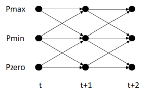
Every arc between two nodes has a well-defined efficiency and profit formula. Hourly commodity prices are plugged in, giving every arc a simple profit (or loss) pre-calculated before the optimization solver runs. We’ll call this step “mapping.” Every scenario will require a new mapping as each time step will have adjusted commodity prices. Arcs connecting Pzero at t to Pmin at t+1 contain the full startup costs.
The magic of the Traveling Salesman Problem is that we do not need to specify an integer number (i.e. 1) of traveling salesmen to travel through our network. This is fortunate for the salesman — the optimizer doesn’t chop him into pieces and send his parts down alternate paths like internet packets. The whole salesman will flow down the best route. Let me clarify: this integer property holds when the profit of each arc is also an integer. Since arcs will typically be weighted by large profits or losses, we can safely round to the nearest integer with no loss of accuracy. This is a big advantage because what typically requires binary state variables within a mixed integer problem can be solved as a linear program (LP) with very efficient algorithms.
With our TSP setup, we can apply other useful constraints on our thermal power station and maintain the linearity of the problem. We can limit the number of starts simply by constraining the maximum times the startup arc in our solution is used. This would be useful if our plant had a contractual service clause with GE or Siemens for a maximum number of starts per year. Likewise, we can constrain the maximum or minimum cumulative production in our period by limiting a weighted sum of the solution arcs chosen. This would be useful if we had volumetric fuel constraints. Moreover, if we need our power station to supply upward flexibility to the grid for a known sub-period we can constrain the plant to run at Pmin for this time.
Implementation
I implemented the above-mentioned power station model in python on one workstation. My code has four functional parts:
- Scenario generation of correlated random forward commodity prices
- Extension of scalar forward prices to vector of hourly spot prices according to own model
- Mapping of the station’s state-space network using the result of the hourly price vectors
- Solving linear program with CPLEX library for python
The linear program must be given to the CPLEX solver in the following form:
Objective:
Minimize sum [- Profit(i) * X(i)], for arc X(i)
Constraints:
sum Xi = 0, for each node except for starting and ending node (what goes into a node must come out)
0 < Xi < 1 (all arcs can take a maximum of 1 traveling salesman)
Depending on the flexibility of the thermal power station that you are modelling, I would recommend a 4- or 8-hour time granularity. You can also customize the network to decrease the slope of specific arcs, for example, to implement a long start-up time. Thus, instead of connecting Pzero at t to Pmin at t+1, connect it to Pmin at t+2, et voila: longer start times.
Next Step: Confiscate the salesman’s crystal ball
Compared to a simple spread option formula with forward prices, such as Margrabe’s Formula with Kirk’s Approximation (which certainly has its place in our toolbox), the TSP-optimized Power Station can capture the fine details of hourly price shape as well as cumulative plant constraints. However, one major shortcoming of the TSP-Station is that the optimization of each price scenario assumes perfect foresight of each arc’s profitability throughout the entire optimization period. (In other words, the traveling salesman knows exactly what the traffic density and petrol price for every leg of his upcoming business trip will be.) This of course will over-estimate the value of the power station, which is very important to remember if you are on the buy side. An important commercial principle that I communicate to clients is to pay only up to the level that you can practically monetize (minus a required cost of capital), not the theoretical value. This will cause you to miss out on a lot of deals, but it will also keep you profitable.
How do we limit our dispatcher’s foresight? We can put our high-priced CPLEX solver back on the shelf and run a modification of Dijkstra’s Algorithm. Dijkstra finds “sufficiently good” paths through the network with limited foresight in polynomial time. The modification we would make to Dijkstra is to extend the foresight to 7 days. This is perfectly reasonable since weather forecasts within one week are accurate, and we know that there’s a distinct intra-week shape to power demand and spot prices. Hence, we already have a good sense of the 7-day price shape. I will leave this implementation for an upcoming article. Thanks for following along.